📡🧬 sig2dna

Symbolic Signal Transformation for Fingerprinting, Alignment, and AI-Based Classification

﹏ ﮩ٨ـﮩﮩ٨ـﮩ٨ـﮩﮩ٨ـ﹏﹏

sig2dna is a Python module that transforms complex 1D, 2D… analytical signals into DNA-like symbolic sequences via morphological encoding. These symbolic fingerprints enable fast alignment, motif recognition, classification, and high-throughput comparison of signals originating from:

GC-MS / GC-FID - 🔍low and🔬high resolution

HPLC-MS - 🔍low and🔬high resolution

NMR / FTIR / Raman / RX

It supports large-scale applications such as identifying unknown substances in ♻️ recycled materials or mixtures containing NIAS (Non-Intentionally Added Substances). 🗜️ Symbolic compression (up to 95%+) enables scalable storage and alignment—and seamless integration with Large Language Models (LLMs).

si2dna Illustrations

🎨 Credits: Olivier Vitrac

📚 This approach was developed and tested as part of the PhD thesis:

Julien Kermorvant, “Concept of chemical fingerprints applied to the management of chemical risk of materials, recycled deposits and food packaging”, AgroParisTech. 2023. https://theses.hal.science/tel-04194172

💡 Note for ND-signals and multi-detector or multi-technique data

sig2dna natively supports signal alignment and comparison across heterogeneous sources. This makes it particularly suited for ND-signals (non-destructive signals) or aggregated data from different detectors or acquisition techniques.

➡️ You can seamlessly concatenate or compare signals originating from different instruments or modes (e.g., UV + MS, GC×GC, LC-FTIR, etc.) — the symbolic coding abstracts away intensity scales and detector-specific artifacts, focusing instead on morphological motifs.

Additional recommendations for 🖼️ 2D and 🗂️ multimodal acquisition systems are given at the end of this document 📄.

📚 Table of Contents

🧩 1| Main Components
🧠 2| Applications
🧬 3| Core Concepts - Overview
🧠 4| Entropy and Distance Metrics
🌀 5 | Sinusoidal Encoding of Symbolic Segments
🔍 6| Baseline Filtering and Poisson Noise Rejection
🧪 7| Synthetic Signal Generation
📦 8| Available Classes
📏 9| Example Workflow
📊 10| Visualization
🔎 11| Motif Detection
🤝 12| Alignment
🧪 13| Examples (unsorted)
📦 14| Installation
💡15| Recommendations
📄 | License
📧 | Contact
📎 |Appendices

🧩 1| Main Components

Class	Description
`DNAsignal`	Encodes numerical signal as symbolic sequence (multi-scale wavelet transform)
`DNAstr`	A symbolic string with alignment, entropy, motif search, plotting, etc.
`DNApairwiseAnalysis`	Computes and visualizes distances, PCoA, clustering, scatter, dendrogram

🧠 2| Applications

High-throughput chemical pattern recognition 🆔, -ˋˏ✄┈┈┈┈
NIAS tracking in complex matrices ⌬,🔔⚠️
AI-compatible signal fingerprints 🫆🔎
Classification of recycled material batches ♻️ 👍
Detection of structural motif distortions (due to overlapping compounds) 🕵🏻
AI-assisted quality control
AI-assisted compliance testing 🍽️

🧬 3| Core Concepts - Overview

Morphology Encoding as a “Genetic” Code. Chemical signals are subjected to signal morphology encoding using continuous, symmetric wavelet transforms. The symbolic sequences are similar to genetic code. It is based on a limited number of letters, symbols appear grouped into motifs which behave like codons As a result, a motif table can be used to recognize n-upplets in ^1^H-NMR, mass spectra, retention times, etc.

Motif Recognition. Searches of substances or typical patterns can be carried out via regular expressions or via transition probabilities (A→Z vs. Z→B vs. A→A) over a sliding window. All operations can be carried out in parallel for efficiency and automated treatment.

Scalable Machine-Learning. High compression ratios enable the efficient storage of millions of chemical signatures.

3.1 Input Signal ➡️

One-dimensional signal objects (NumPy-based)
Supports synthetic and experimental sources

S = signal.from_peaks(...)

🟥

3.2 Wavelet Transform 〰

A Mexican hat (Ricker) wavelet is used:

\[\psi_s(t) = \left(1 - \frac{t^2}{s^2}\right)e^{-\frac{t^2}{2s^2}}\]

The Continuous Wavelet Transform (CWT) of a signal \(x(t)\) is:

\[W_s(t) = x(t)*\psi_s(t) = \int x(\tau) \cdot \psi_s(t - \tau) \, d\tau\]

where \(s\) is the scale parameter (typically powers of two, e.g., \(s = 2^n\)) and \(*\) the convolution operator.

🟪

3.3 Relationship of \(W\_s(t)\) with the second derivative \(x''(t)=\frac{\partial^2 x(t)}{\partial t^2}\)

Applying the Ricker wavelet (second derivative of a Gaussian) to the signal \(x(t)\) via convolution (i.e., CWT) is equivalent to computing the second derivative of \(x(t)\) smoothed by the Gaussian kernel \(g\_s(t)\):

\[W_s(t) = x(t)*\psi_s(t) = x(t) * g''(t) = x''(t) * g(t)\]

Click here for the demonstration

The convolution of \(x(t)\) with the second derivative of \(g(t)\) is:

\((x * g'')(t) = \int\_{-\infty}^{\infty} x(\tau) g''(t - \tau) \, d\tau\)

We perform a change of variable: let \(u = t - \tau\), so \(\tau = t - u\) and \(d\tau = -du\). This gives:

\((x * g'')(t) = \int\_{-\infty}^{\infty} x(t - u) g''(u) \, du\)

Now consider the convolution of the second derivative of \(x(t)\) with \(g(t)\):

\((x'' * g)(t) = \int\_{-\infty}^{\infty} x''(\tau) g(t - \tau) \, d\tau\)

Again, perform the change of variable \(u = t - \tau\), yielding:

\((x'' * g)(t) = \int\_{-\infty}^{\infty} x''(t - u) g(u) \, du\)

Now integrate by parts twice:

First integration by parts (assuming \(g(u) \to 0\) and \(x'(t - u) \to 0\) as \(u \to \pm \infty\)):

\(\int x''(t - u) g(u) \, du = - \int x'(t - u) g'(u) \, du\)

Second integration by parts:

\(-\int x'(t - u) g'(u) \, du = \int x(t - u) g''(u) \, du\)

Which yields:

\((x'' * g)(t) = \int x(t - u) g''(u) \, du = (x * g'')(t)\)

🟦

3.4 Symbolic Encoding 🔡

Each segment of the wavelet-transformed signal is encoded into one of the symbolic codes corresponding to the table of variation \(\text{sign}\left(\frac{\partial}{\partial t}W\_s(t)\right)\) and \(\text{sign}\left(W\_s(t)\right)\).

Symbol: \(\ell\_i\)	Variation	Description
`A`	-↗+	Increasing crossing from − to + (zero-crossing)
`B`	-↗-	Increasing negative
`C`	+↗+	Increasing positive
`X`	+↘+	Decreasing positive
`Y`	-↘-	Decreasing negative
`Z`	+↘-	Decreasing crossing from + to − (zero-crossing)
`_`	──	Flat or noise segment

Each segment stores its width, height, and position.

The full-resolution symbolic sequence is reconstructed by interpolating or repeating these symbols proportionally to their span. A quantitative pseudo-inverse is proposed to reconstruct chemical signals from their code.

🟩

3.5 Symbolic Compression 🗜️

Symbolic sequences can be compressed and encoded at full resolution via:

dna.encode_dna()
dna.encode_dna_full(resolution="index")

Resulting in DNA-like sequences like:

"YYAAZZBB_YAZB"

🟨

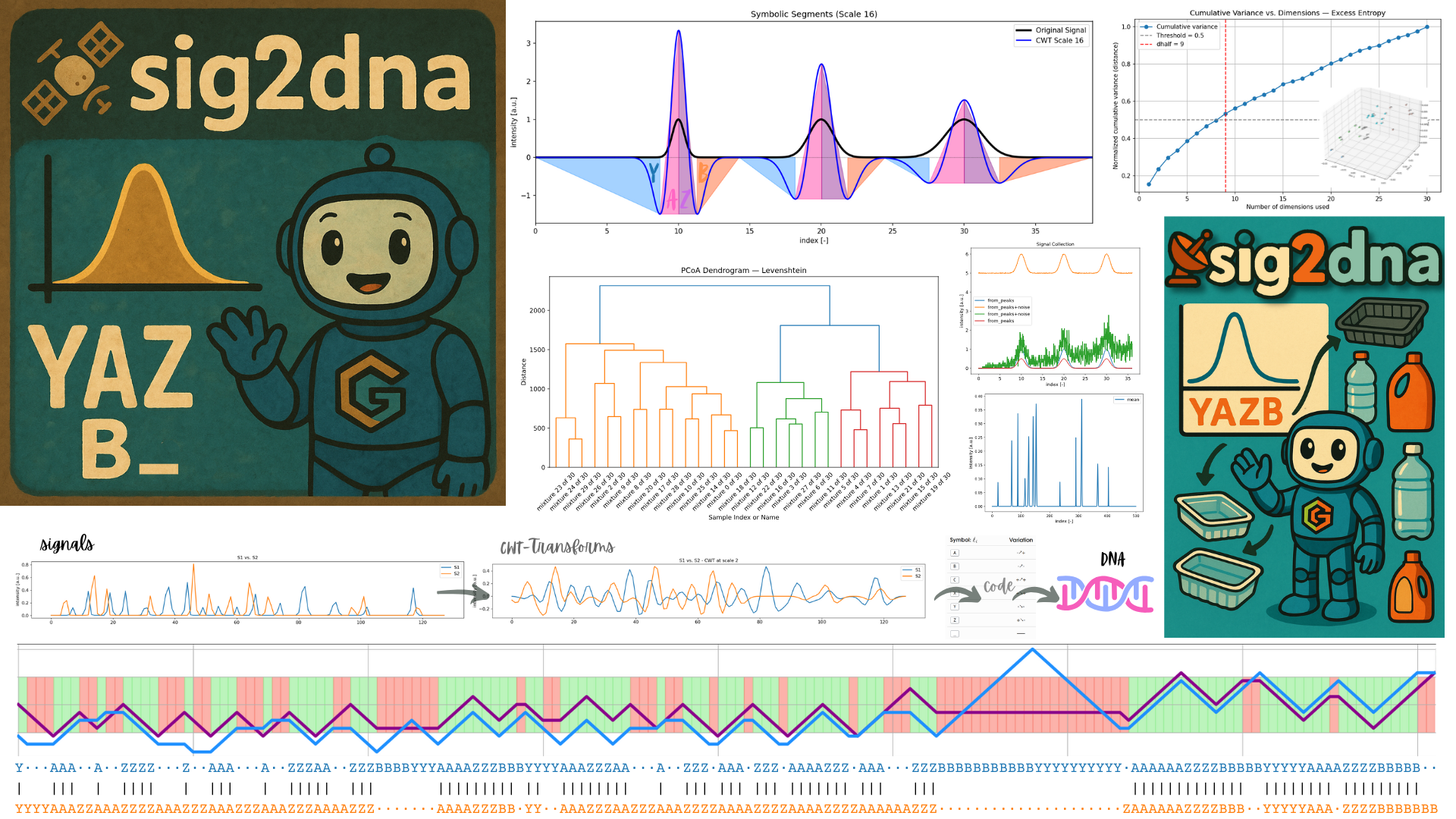
3.6 Structural Meaning (e.g., `YAZB` Motif)

A single Gaussian peak transformed via the Ricker wavelet results in:

Y: rising pre-lobe ꒷꒦꒷꒦꒷꒦꒷꒦꒷꒦꒷
A: left inflection (− to + crossing)
Z: right inflection (+ to − crossing)
B: trailing decay

The YAZB motif is a symbolic map of the Ricker wavelet transform (CWT) of a Gaussian. An alteration of the pattern reveals overlapping Gaussians , asymmetric signals or more generally interactions and interferences.

🟧

3.7 Interpretation When Gaussians Overlap 🌈⃤

When two Gaussians overlap, especially at close proximity or with different amplitudes:

The central peak becomes asymmetric.
The Ricker transform becomes a superposition of two wavelets.
This causes:
- Emergence of extra inflection points,
- Distortion of the clean YAZB sequence,
- Insertion of intermediary motifs (e.g., repeating A-Z transitions, shortened or elongated lobes),
- Possible merging of YAZB motifs or partial truncation.

So changes in the symbolic code structure directly reflect signal interference, i.e., nonlinearity in overlapping peaks.

🧠 4| Entropy and Distance Metrics

Sig2dna implements several metrics to evaluate the similarity of coded chemical signals. Alignment is essential to compare them while respecting order. It is performed via global/local pairwise alignment using difflib or Biopython. Excess Entropy and Jensen-Shannon are best choices in the presence of complex mixtures by enabling the detection of small structural changes.

Distance	Sensitive to	Based on	Alignment needed	Suitable for
Excess Entropy	Symbol order	Shannon entropy	✅ Yes	Structural motif similarity
Jensen-Shannon	Symbol usage	Probability dist.	❌ No	Profile similarity (e.g., peak types)
Levenshtein	Edit steps	Insertion/Deletion	✅ Yes	Sequence-level variation
Jaccard	Pattern sets	Motif occurrences	❌ No	Motif overlap, Motif density map

4.1 Shannon Entropy ⚀⚁⚂⚃⚄⚅

Entropy provides a robust, physics-informed metric for morphological comparisons. For a symbolic sequence \(X\), it reads:

\[H(X) = -\sum_i p(\ell_i) \log_2 p(\ell_i)\]

where \(p(\ell\_i)\) is the frequency of letter \(l\_i\) in the sequence \(X\).

Entropy \(H\) is an extensive quantity verify additivity properties for independent sequences. Its value is accumulated between structured and low structured regions. Entropy is invariant under translation and stable under small perturbations, especially when using symbolic codes rather than raw intensities. This makes it ideal for comparing:

Signals with shifts in baseline
Morphologically similar but intensity-scaled signals
Partially distorted sequences (e.g., from mixtures or degradation)

🔴

4.2 Aligned sequences and Excess Entropy Distance ↔️

Let \(A\) and \(B\) be two symbolic sequences (DNAstr) representing two signals. After alignment (e.g., via global/local pairwise alignment using difflib or Biopython), we obtain:

\(\tilde{A}\): aligned version of \(A\) (with possible gap insertions)
\(\tilde{B}\): aligned version of \(B\)
\(\tilde{A} * \tilde{B}\): a new sequence formed by pairing corresponding symbols (possibly with gaps)

Given sequences \(A\) and \(B\), the mutually exclusive information or excess entropy is defined as:

\[D_{\text{excess}}(A, B) = H(A) + H(B) - 2 H(\tilde{A} * \tilde{B})\]

where:

\(H(A)\) and \(H(B)\) are the Shannon entropies of the original sequences
\(H(\tilde{A} * \tilde{B})\) is the Shannon entropy of the aligned signal pairs (treated as “joint letters”)

🟠

4.3 Jensen-Shannon Distance ↔️

Let \(P\) and \(Q\) be the empirical frequency distributions of symbolic letters in two DNA-like coded signals \(A\) and \(B\), respectively. That is:

\(P = {p\_\ell}\) where \(p\_\ell = \frac{\text{count of symbol } \ell \text{ in } A}{|A|}\)
\(Q = {q\_\ell}\) where \(q\_\ell = \frac{\text{count of symbol } \ell \text{ in } B}{|B|}\)

Let \(M\) be the average distribution:

\[M = \frac{1}{2}(P + Q)\]

Then, the Jensen–Shannon distance between \(P\) and \(Q\) is defined as:

\[D_{\text{JS}}(P, Q) = \sqrt{ \frac{1}{2} D_{\text{KL}}(P \| M) + \frac{1}{2} D_{\text{KL}}(Q \| M) }\]

where \(D\_{\text{KL}}\) is the Kullback-Leibler divergence:

\[D_{\text{KL}}(P \| M) = \sum_\ell p_\ell \log_2 \left( \frac{p_\ell}{m_\ell} \right)\]

and \(m\_\ell\) is the frequency of symbol \(\ell\) in the average distribution \(M\).

4.3.1 Interpretation 💡

The Jensen–Shannon distance quantifies how different the symbol usage is between two signals, ignoring the order in which the symbols appear.
It is bounded between 0 and 1, symmetric, and always finite (even when some symbols are missing in one sequence).
A value of 0 indicates identical symbol distributions, while 1 indicates completely disjoint symbol usage.

4.3.2 Use Cases 🧪

Robust against misalignment or noise: two signals with similar overall composition but different positions will still score low JSD.
Useful for clustering symbolic signals by type or composition, regardless of temporal structure.
Complementary to entropy or edit-based distances, which capture positional or morphological changes.

🟡

4.4 Jaccard Motif Distance 🔍

The Jaccard distance measures the similarity between two symbolic signals by comparing the sets of motifs (short symbolic substrings) they contain, without requiring alignment. It is particularly suited for identifying common structural patterns across signals, regardless of their order or spacing.

Given two sequences \(A\) and \(B\), and a set of motifs \(\mathcal{M}\) of length \(k\) (typically 3–5 characters), we define:

\(\mathcal{M}(A)\): set of motifs found in \(A\)
\(\mathcal{M}(B)\): set of motifs found in \(B\)

Then the Jaccard distance is defined as:

\[D_{\text{Jaccard}}(A, B) = 1 - \frac{|\mathcal{M}(A) \cap \mathcal{M}(B)|}{|\mathcal{M}(A) \cup \mathcal{M}(B)|}\]

4.4.1 Key Features:

✅ No alignment needed — motif presence is evaluated globally
🔍 Sensitive to local patterns — detects repeated or shared symbolic structures
📈 Sparse and interpretable — suitable for heatmaps and clustering

4.4.2 Implementation Notes:

Motifs are extracted using a sliding window of fixed length (default: k=4)
Symbol sequences are assumed to be from the encoded DNAstr outputs
Motif sets are hashed to speed up large comparisons
Jaccard scores are computed pairwise across a collection of symbolic sequences

This metric is especially useful when:

You expect common substructures across signals
Signals may differ in length or alignment is unreliable
You want to create density maps of motif usage or explore structural similarity clusters

Here is the complete, cleanly formatted README.md documentation section for the new sinusoidal encoder/decoder functions added to sig2dna, including appropriate emojis and explanations:

🌀 5 | Sinusoidal Encoding of Symbolic Segments

sig2dna integrates a transformer-style positional encoding for symbolic segments, enabling conversion of morphological features into fixed-size vectors. This provides a compact, AI-ready representation of:

⏱️ Position (\(x\_0\))
📏 Width (\(\Delta x\))
📶 Amplitude (\(\Delta y\))

💡 This mechanism replaces long repetitions of letters by a numerically invertible vector encoding, useful for clustering, attention-based models, or compressed storage.

5.1 Mathematical Basis 📐

Let \(t \in \mathbb{R}\) be a scalar quantity (e.g., position, width, or height). The sinusoidal encoding \(\mathbf{f}(t) \in \mathbb{R}^d\) is defined by:

\[\begin{split}\begin{aligned} f_{2k}(t) &= \sin\left(\frac{t}{r^k}\right), \\ f_{2k+1}(t) &= \cos\left(\frac{t}{r^k}\right), \end{aligned} \quad \text{for } k = 0, \dots, \frac{d}{2}-1\end{split}\]

where:

\(r = N^{2/d}\) is a frequency base (default: \(N = 10000\))
\(d\) is the number of embedding dimensions for the feature (default: \(d = 32\))
Each encoded feature (position, width, amplitude) gets its own \(d\)-vector

Then the full vector for one symbolic segment becomes:

\[\mathbf{v} = [\mathbf{f}(x_0) \, \| \, \mathbf{f}(\Delta x) \, \| \, \mathbf{f}(\Delta y)] \in \mathbb{R}^{3d}\]

These vectors are computed for each letter (A, B, …, Z) and grouped accordingly.

This encoding maps any scalar value \(t\) (e.g., ⏱️, 📏, 📶) onto periodic functions. Due to the nature of sine and cosine, this representation is:

translation-equivariant for local displacements (relative order and spacing are preservd),

periodic, so absolute positions wrap with ambiguity (exact localization may be lossy).

The key mathematical identity is:

\[f(t + \Delta t) = \mathrm{diag}(f(\Delta t)) \cdot f(t) \]

>
>
> 👉 **shifting** a position $t$ by $\Delta t$ corresponds to a **linear transformation** of its embedding.
>
> ⚠️ To enable **invertibility**, we restrict $x_0$ within a known range $[0, L]$ with resolution determined by $N$ (current implementation), or add explicit absolute anchor

🔵〰️〰️⚪️〰️〰️〰️🔴

### 5.2  Decoding implementation 🗝️ 

- **Encoding**: $t \mapsto [\sin(t/r_k), \cos(t/r_k)]_{k=0}^{d/2 - 1}$

- **Decoding**:
- Convert $\sin$, $\cos$ pairs into $z_k = \cos + i\sin = e^{ix/r_k}$
  
- Unwrap $\angle(z_k)$ → gives $\theta_k \approx t/r_k$
  
- Fit $t$ via least-squares:

```{math}
x\_i = \frac{\sum\_k \theta\_{ik} \cdot \frac{1}{r\_k}}{\sum\_k \left(\frac{1}{r\_k}\right)^2}

Robust, differentiable, and avoids scalar-local minima traps.

Four decoders have been implemented 🔧:

Method

Description

Stability

'least_squares'

Fast, phase-unwrapped projection

✅ Excellent

'svd'

SVD-regularized LSQ for robust inversion

✅ Excellent

'optimize'

Scalar optimization (slow, fragile)

❌ Unstable

'naive'

Mean of phase-projected values (quick + dirty)

❌ Wrong shifts

Rules of Thumb 🔧:

Option

Action

Effect

Use scaling

Normalize input to [0, 10]

Accurate decoding for wide range

Reduce N

Use e.g. N = 1000

Higher range support

🔷〰️〰️🔷〰️〰️〰️🔷

5.3 `sinencode_dna()` – Letter-wise Sinusoidal Encoder 🔡

Encodes all symbolic segments at selected scale(s) into sinusoidal vectors, grouped by letter (A, Z, B, etc.).

dna.sinencode\_dna(scales=[4], d\_part=32)

🔧 Stored outputs:

self.code_embeddings_grouped:

{
  4: {
    "A": np.ndarray (n\_A, 96),
    "Z": np.ndarray (n\_Z, 96),
    ...
  }
}

self.code_embeddings_meta: Metadata required for reconstruction:

{
  "sampling\_dt": 0.1,
  "x\_label": "RT",
  "x\_unit": "min",
  "y\_label": "Intensity",
  "y\_unit": "a.u.",
  "name": "GC-MS peak trace",
  "scales": [4],
  "d\_part": 32,
  "N": 10000
}

🔶〰️〰️🔶〰️〰️〰️🔶

5.4 `sindecode_dna(...)` – Static Decoder to DNAsignal 🔁

Reconstructs a new DNAsignal instance from sinusoidal embeddings:

reconstructed = DNAsignal.sindecode\_dna(
    grouped\_embeddings = dna.code\_embeddings\_grouped,
    meta\_info = dna.code\_embeddings\_meta
)

🧬 Returns a complete DNAsignal object with:

reconstructed codes[scale] dictionaries:
- letters, widths, heights, iloc, xloc, dx
empty signal (since waveform cannot be recovered from symbol encoding alone)

🧠 Ideal for:

Embedding symbolic sequences for AI/ML workflows
Comparing motifs without repeating long letters
Visualizing symbolic structure in latent spaces

⭐〰️〰️⭐〰️〰️〰️⭐

5.5 Summary and error estimation \(\varepsilon = |\hat{t} - t|\) 💬

Each scalar \(t\) (like \(x_0\) or \(\Delta x\)) is encoded as:

\[\mathbf{f}(t) = \left[ \sin\left(\frac{t}{r^0}\right), \cos\left(\frac{t}{r^0}\right), \dots, \sin\left(\frac{t}{r^{d/2-1}}\right), \cos\left(\frac{t}{r^{d/2-1}}\right) \right]\]

with \(r = N^{2/d}\), typically \(N = 10000\), and \(d \sim 32\).

In decoding, we estimate \(t\) by averaging multiple phase inversions:

\[\hat{t} \approx \frac{1}{d/2} \sum\_{k=0}^{d/2 - 1} r^k \cdot \theta\_k, \quad \text{where } \theta\_k = \arctan\left( \frac{\sin(t/r^k)}{\cos(t/r^k)} \right)\]

Let \(L\) be the maximum span of \(t\) values to encode (e.g., total signal length), and \(d\) the embedding size (e.g., 32). Then:

For \(k=0\) (highest freq), \(\text{period}_0 \sim 2\pi\)
For \(k = d/2 - 1\), \(\text{period}_k \sim 2\pi N\)

So the resolution behaves like:

\[\varepsilon \sim \frac{L}{N}\]

where \(N\) is the frequency base and \(L\) is the range of \(t\) values being encoded (e.g., max segment length or signal length)

Feature	Value
Error scales	\(\varepsilon \sim L / N\)
Depends on	Signal span \(L\), base \(N\)
Tunable by	Increasing \(d\) or \(N\)
Accuracy	Typically \(<0.1%\) %of signal range (\(L=500\) and \(N=10^4\) gives \(\varepsilon \approx \frac{500}{10000} = 0.05\) )
Robustness	Stable across most morphologies

The errors are acceptable for:

Motif alignment
Classifiers
Density maps
Latent embeddings

🔍 6| Baseline Filtering and Poisson Noise Rejection

The Ricker wavelet \(\psi_s(t)\) used in sig2dna is mathematically the second derivative of a Gaussian kernel. As such, applying the Continuous Wavelet Transform (CWT) with \(\psi_s(t)\) is equivalent to performing a second-order differentiation of the signal \(x(t)\) followed by a Gaussian smoothing, where the scale parameter \(s\) controls the bandwidth.

This structure makes the CWT intrinsically robust to low-frequency noise, baseline drifts, and stationary random noise (such as column bleeding in GC). Moreover, the symmetry of \(\psi_s(t)\) ensures suppression of linear trends, enhancing signal clarity without distorting peak structures.

For ideal Gaussian-shaped peaks, the optimal CWT response is obtained when the scale \(s\) matches the peak’s width at its inflection points, which corresponds to half-height for a Gaussian. This is where the symbolic motif YAZB is most cleanly detected.

However, on real-life signals, maximizing noise rejection by increasing \(s\) can blur peak details. Preserving the morphological fidelity of peaks while ensuring their detectability requires operating near the optimal scale, not beyond it. To this end, sig2dna integrates a robust preprocessing methodology tailored for signals acquired through accumulation or integration (i.e., counting statistics), such as total ion counts in mass spectrometry or spectroscopic intensities.

Step 1 — Median Baseline Subtraction ﹏𓊝﹏

Let \(x(t)\) be the input signal. We compute a moving median over a window of width \(w\):

\[\text{baseline}(t) = \text{median}\left[x(t - w/2), \dots, x(t + w/2)\right]\]

Then, apply a non-negative correction:

\[x\_b(t) = \max\left(0,\, x(t) - \text{baseline}(t)\right)\]

🏻‎🏼‎🏽‎🏾🏿

Step 2 — Poisson Noise Estimation ▶︎ ၊၊||၊|။|||| |

From the baseline-corrected signal \(x_b(t)\):

Compute the local mean \(\mu(t)\) and standard deviation \(\sigma(t)\) using a uniform filter.
Estimate the coefficient of variation:

\[\text{cv}(t) = \frac{\sigma(t)}{\mu(t)}\]

Assuming Poisson noise, infer the local Poisson parameter:

\[\lambda(t) = \frac{1}{\text{cv}(t)^2}\]

🏻‎🏼‎🏽‎🏾🏿

Step 3 — Bienaymé–Tchebychev Thresholding 🗑️

To reject noise, use a threshold \(T(t)\) derived from \(\lambda(t)\):

\[T(t) = k \cdot \sqrt{10 \lambda(t) \Delta t}\]

Filtered signal is then:

\[\begin{split}x\_{bf}(t) = \begin{cases} x\_b(t) & \text{if } x\_b(t) > T(t) \\ 0 & \text{otherwise} \end{cases}\end{split}\]

🧪 7| Synthetic Signal Generation

Synthetic signals are modeled as a sum of Gaussian/Lorentzian/Triangle peaks. For Gaussian, they read

\[s(t) = \sum\_{i} h\_i \cdot \exp\left(-\left(\frac{t - \mu\_i}{0.6006 \cdot w\_i}\right)^2\right)\]

where:

\(h_i\): peak height
\(\mu_i\): center
\(w_i\): peak width (calibrated to Full Width Half Maximum)

This is used to:

Reconstruct symbolic segments
Generate artificial mixtures
Simulate motifs for clustering or ML training
Parses sequences into YAZB motif candidates (Mass spectra)

📦 8| Available Classes

Module sig2dna_core.signomics.py

Class Name	Description
`generator`	Peak shape generator: Gaussian, Lorentzian, triangle
`peaks`	Peak library with synthesis, parameter control, and arithmetic operations
`signal`	1D signal class with plotting, peak summation, transformations, and noise
`signal_collection`	Wrapper for multi-signal analysis: mean, sum, scaling, alignment, synthesis
`DNAstr`	Symbolic sequence class with entropy, motif search, edit distances
`DNAsignal`	Symbolic encoding/decoding from signals (DNA-like)
`DNApairwiseAnalysis`	Tools for clustering, dimensionality reduction, dendrograms, visual metrics
`DNAsignal_collection`	Wrapper for 2D, nD DNAsignals
`SinusoidalEncoder`	Encoder/decoder for symbolic and numeric data using sinusoidal projections
`DNACodes`	Dictionary-like symbolic representation of triplet codes (letter, width, height)
`DNAFullCodes`	Dictionary-based encoder for resolution-based symbolic repetition

Class Inheritance Diagram

        graph TD;
DNACodes
DNAFullCodes
DNApairwiseAnalysis
DNAsignal
DNAsignal_collection
DNAstr
SinusoidalEncoder
generator
peaks
signal
signal_collection
UserDict --> DNACodes
dict --> DNAFullCodes
list --> DNAsignal_collection
list --> signal_collection
object --> DNApairwiseAnalysis
object --> DNAsignal
object --> SinusoidalEncoder
object --> generator
object --> peaks
object --> signal
str --> DNAstr

📏 9| Example Workflow

from signomics import DNAsignal

# Load and encode
D = DNAsignal(S, encode=True)
D.encode\_dna()
D.encode\_dna\_full()

# Visualize
D.plot\_codes(scale=4)

# Entropy and distances
entropy = D.get\_entropy(scale=4)
analysis = DNAsignal.\_pairwiseEntropyDistance([D1, D2, D3], scale=4)

📊 10| Visualization

signal.plot(), signal_collection.plot() : plot signals
DNAsignal.plot_signals(): Original + CWT overlay
DNAsignal.plot_transforms(): plot transformed signals a collection of signals
DNAsignal.plot_codes(scale=4): Colored triangle segments
DNAstr.plot_mask: plot alignment mask
DNAstr.plot_alignment: plot aligned codes as reconstructed signals
DNApairwiseAnalysis.plot_dendrogram(), scatter3d(), scatter(), heatmap, dimension_variance_curve: Cluster and distance views

🔎 11| Motif Detection

Pattern search: ꒷꒦꒷꒦꒷꒦꒷꒦꒷꒦꒷

listPat=D.codes[4].find("YAZB")
listPat[0].to\_signal().plot() # show the first match as a signal

Extract and plot motifs: ▌│█║▌║▌║

D.codesfull[4].extract\_motifs("YAZB", minlen=4, plot=True)

🤝 12| Alignment

☴ Fast symbolic alignment:⛓️⏱️

D1.codes[4].align(D2.codes[4], engine="bio")
D1.codes[4].wrapped\_alignment()
D1.html\_alignment()
D1.plot\_alignment()

🧪 13| Examples (unsorted)

from sig2dna\_core.signomics import peaks, signal\_collection, DNAsignal

# 1. Peak creation and basic signals 🏔️
p = peaks()
p.add(x=10, w=2, h=1)
p.add(x=20, w=2, h=1)
s = p.to\_signal()
s.plot()

# 2. Signal collection 🗃️
s\_noisy = s.add\_noise("gaussian", scale=0.01, bias=5)
s\_scaled = s * 0.5
coll = signal\_collection(s, s\_noisy, s\_scaled)
s\_mean = coll.mean()
s\_mean.plot(label="Mean")

# 3. Synthetic mixtures 🥣
S, pS = signal\_collection.generate\_synthetic(n\_signals=12, n\_peaks=1, ...)
Sfull = S.mean()
dna = DNAsignal(Sfull)
dna.compute\_cwt()
dna.encode\_dna\_full()
dna.plot\_codes(scale=4)

# 4. Alignment of encoded sequences 🧬🧬
A = dna.codesfull[4]
B = dna.codesfull[2]
A.align(B)
A.html\_alignment()
A.plot\_alignment()

# 5. Extract motifs (e.g., YAZB segments ⚗️
pA = A.find("YAZB")
pAs = signal\_collection(*[s.to\_signal() for s in pA])
pAs.plot()

# 6. Classification from mixtures 🏁
Smix, pSmix, idSmix = signal\_collection.generate\_mixtures(...)
dnaSmix = Smix.\_toDNA(scales=[1,2,4,8,16,32])

# 7. Excess entropy distance & clustering 🎲
D = DNAsignal.\_pairwiseEntropyDistance(dnaSmix, scale=4, engine="bio")
D.name = "Excess Entropy"
D.dimension\_variance\_curve()
D.select\_dimensions(10)
D.plot\_dendrogram()
D.scatter3d(n\_clusters=5)

# 8. Jaccard motif distance ↔️
J = DNAsignal.\_pairwiseJaccardMotifDistance(dnaSmix, scale=4)
J.name = "YAZB Jaccard"
J.dimension\_variance\_curve()
J.select\_dimensions(10)
J.plot\_dendrogram()
J.scatter3d(n\_clusters=5)

📦 14| Installation

The sig2dna toolkit is composed of two core modules that must be used together:

🧩 Module	Description
🧬 `sig2dna_core.signomics`	Core module implementing symbolic transformation, wavelet coding, and signal comparison (compact code, >7 Klines)
🖨️ `sig2dna_core.figprint`	Utility module for saving and exporting Matplotlib figures (PDF, PNG, SVG)

Recommended File Structure 🛠

For simplicity and consistency, it is recommended to use both modules from a local subfolder (e.g., sig2dna_core) within your working directory. You can clone or place the source files accordingly:

📂 sig2dna/                <- your working directory
│
├── 📂 sig2dna\_core/       <- folder for core modules
│   ├── 🖨️ figprint.py     <- figure saving utilities
│   └── 🧬 signomics.py    <- main symbolic signal processing module (>4 Klines)
│
├── 📂 sig2dna\_tools/       <- folder for tools (not included in this release)
│
├── 📁 images/             <- output folder for saved figures (PDF, PNG, SVG)
│
├── 📝 yourscript.py       <- your script using sig2dna\_core modules
│
├── 📄 test\_signomics.py      <- minimal test and plotting script
├── 📄 casestudy\_signomics.py <- in-depth classification and clustering example
├── 📜 LICENSE
└── 📑 README.md

Import Example 📥

In your scripts, import the components directly:

from sig2dna\_core.signomics import peaks, signal\_collection, DNAsignal

Dependencies 📦

The project relies only on standard scientific Python libraries and a few well-known optional packages. All can be installed with conda or pip:

conda install pywavelets seaborn scikit-learn
conda install -c conda-forge python-Levenshtein biopython

Or using pip:

pip install PyWavelets seaborn scikit-learn python-Levenshtein biopython

✅ No installation script is needed; simply place the module files in your working directory and ensure the structure above is respected.

💡15| Recommendations

Substance Identification and Library Matching 🔍

sig2dna includes signal reconstruction capabilities from the symbolic code, allowing for approximate substance identification against reference libraries.

However, when precise identification is required:

✅ It is preferable to transform the mass spectra of reference substances using sig2dna and compare them directly to the coded signal.

This enables symbol-level matching, which is more robust to noise, shifts, and peak distortion than traditional numerical similarity or library lookup.

📄 | License

MIT License — 2025 Olivier Vitrac

📧 | Contact

Author: Olivier Vitrac Contact: olivier.vitrac@gmail.com Version: 0.43 (2025-06-13)

Sig2dna is part of the Generative Simulation initiative 🌱: building modular, interpretable AI-ready tools for scientific modeling.

📎 |Appendices

🧩 | Methods Table (module: `sig2dna.signomics`)

Class	Method	Docstring First Paragraph	# Lines	version
(module-level)	`import_local_module`	Import a module by name from a file path relative to the calling module.	37	0.51
`DNACodes`	`__init__`	Initialize self. See help(type(self)) for accurate signature.	4	0.51
`DNACodes`	`plot`	Plot method for DNACodes: visualizes encoded vectors or symbolic segment distribution.	57	0.51
`DNACodes`	`sindecode`	Decode sinusoidally embedded codes grouped by letter into symbolic segment structure.	24	0.51
`DNACodes`	`sinencode`	Encode symbolic segments at each scale using sinusoidal encoding grouped by letter.	22	0.51
`DNACodes`	`summary`	Print the number of encoded vectors or symbolic segments per scale.	12	0.51
`DNAFullCodes`	`__init__`	Initialize self. See help(type(self)) for accurate signature.	4	0.51
`DNAFullCodes`	`__repr__`	Return repr(self).	2	0.51
`DNAFullCodes`	`__str__`	Return str(self).	2	0.51
`DNAFullCodes`	`plot`	Plot method for DNAFullCodes: visualizes encoded vectors or DNA string composition.	53	0.51
`DNAFullCodes`	`plot_unwrapped_matrix`	Plot each letter’s encoded vector in the abstract embedding space (d-space). One curve per letter, one subplot per scale.	38	0.51
`DNAFullCodes`	`sindecode`	Sindecode method	11	0.51
`DNAFullCodes`	`sinencode`	Sinencode method — encodes each letter in the DNAFullCodes as a set of sinusoidal embeddings.	45	0.51
`DNAFullCodes`	`summary`	Return a brief summary of the full codes per scale.	10	0.51
`DNAFullCodes`	`unwrap_letters_to_matrix`	Assemble all encoded letter vectors into a matrix of shape (n_letters, d_model) for each scale.	38	0.51
`DNApairwiseAnalysis`	`__init__`	Initialize self. See help(type(self)) for accurate signature.	10	0.51
`DNApairwiseAnalysis`	`__repr__`	Return repr(self).	7	0.51
`DNApairwiseAnalysis`	`__str__`	Return str(self).	2	0.51
`DNApairwiseAnalysis`	`best_dimension`	Determine optimal dimension by maximizing silhouette score.	16	0.51
`DNApairwiseAnalysis`	`cluster`	Assign cluster labels from linkage matrix.	5	0.51
`DNApairwiseAnalysis`	`compute_linkage`	Compute hierarchical clustering.	6	0.51
`DNApairwiseAnalysis`	`dimension_variance_curve`	Computes the cumulative explained variance (based on pairwise distances) as a function of the number of dimensions used (from 1 to n-1). Optionally plots the curve and the point where the threshold (default 0.5) is reached.	46	0.51
`DNApairwiseAnalysis`	`get_cluster_labels`	Returns cluster labels from hierarchical clustering. If not computed yet, computes linkage.	20	0.51
`DNApairwiseAnalysis`	`heatmap`	Plot heatmap of pairwise distances.	9	0.51
`DNApairwiseAnalysis`	`load`	Load analysis from file.	5	0.51
`DNApairwiseAnalysis`	`pcoa`	Perform Principal Coordinate Analysis (PCoA).	7	0.51
`DNApairwiseAnalysis`	`plot_dendrogram`	Plot dendrogram from linkage matrix.	14	0.51
`DNApairwiseAnalysis`	`reduced_distances`	Recompute distances on selected subspace.	4	0.51
`DNApairwiseAnalysis`	`save`	Save current analysis to file.	4	0.51
`DNApairwiseAnalysis`	`scatter`	2D scatter plot in selected dimensions with optional cluster-based coloring.	40	0.51
`DNApairwiseAnalysis`	`scatter3d`	3D scatter plot in selected dimensions with optional cluster-based coloring.	38	0.51
`DNApairwiseAnalysis`	`select_dimensions`	Update active dimensions.	8	0.51
`DNAsignal`	`__init__`	Initialize DNAsignal with a signal object or 1D array.	58	0.51
`DNAsignal`	`__repr__`	Return repr(self).	6	0.51
`DNAsignal`	`__str__`	Return str(self).	2	0.51
`DNAsignal`	`_get_letter`	Determine letter based on monotonicity and signal range.	31	0.51
`DNAsignal`	`_get_triangle_from_letter`	returns the triangle (counter-clockwise, x are incr)	27	0.51
`DNAsignal`	`_pairwiseEntropyDistance`	Calculate excess-entropy pairwise distances.	52	0.51
`DNAsignal`	`_pairwiseJaccardMotifDistance`	Compute pairwise Jaccard distances based on motif presence across symbolic DNAstr sequences.	102	0.51
`DNAsignal`	`_pairwiseJensenShannonDistance`	Calculate pairwise Jensen-Shannon distances between DNAstr codes at a given scale.	45	0.51
`DNAsignal`	`_pairwiseLevenshteinDistance`	Compute pairwise Levenshtein distances between codes at a given scale.	61	0.51
`DNAsignal`	`align_with`	Align symbolic sequences and compute mutual entropy.	27	0.51
`DNAsignal`	`apply_baseline_filter`	Apply baseline filtering using moving median and local Poisson-based thresholding.	58	0.51
`DNAsignal`	`compute_cwt`	Compute Continuous Wavelet Transform (CWT) using the Mexican Hat wavelet.	46	0.51
`DNAsignal`	`encode_dna`	Encode each transformed signal into a symbolic DNA-like sequence of monotonic segments.	67	0.51
`DNAsignal`	`encode_dna_full`	Convert symbolic codes into DNA-like strings by repeating letters proportionally to their span.	78	0.51
`DNAsignal`	`entropy_from_string`	return the entropy of a string	5	0.51
`DNAsignal`	`find_sequence`	Find occurrences of a specific letter pattern in encoded sequence.	9	0.51
`DNAsignal`	`get_code`	Retrieve encoded data for a specific scale.	3	0.51
`DNAsignal`	`get_entropy`	Calculate Shannon entropy for encoded signal.	5	0.51
`DNAsignal`	`has`	Check if a DNA encoding exists for the specified scale.	22	0.51
`DNAsignal`	`normalize_signal`	Normalize the internal signal using one of several strategies that ensure positivity.	18	0.51
`DNAsignal`	`plot_codes`	Plot the symbolic DNA-like encoding as colored triangle segments.	77	0.51
`DNAsignal`	`plot_scalogram`	Plot a scalogram with two subplots: - Top: colored image of CWT coefficient amplitudes - Bottom: line curves of selected scales	34	0.51
`DNAsignal`	`plot_signals`	Plot signals.	13	0.51
`DNAsignal`	`plot_transforms`	Plot the stored CWT-transformed signals as a signal collection.	13	0.51
`DNAsignal`	`print_alignment`	print aligned sequences	11	0.51
`DNAsignal`	`pseudoinverse`	Approximate signal reconstruction via pseudo-inverse using stored CWT coefficients.	64	0.51
`DNAsignal`	`reconstruct_aligned_string`	Fast reconstruction of aligned signals	9	0.51
`DNAsignal`	`reconstruct_signal`	Reconstruct the signal from symbolic features (e.g., YAZB).	31	0.51
`DNAsignal`	`sindecode_dna`	Decode sinusoidal grouped embeddings into a DNACodes structure.	27	0.51
`DNAsignal`	`sinencode_dna`	Encode `self.codes` into sinusoidal embeddings (grouped by letter).	15	0.51
`DNAsignal`	`sinencode_dna_full`	🌀 Encode full-resolution DNA-like strings into sinusoidal embeddings grouped by letter.	37	0.51
`DNAsignal`	`sparsify_cwt`	Sparsify CWT coefficients by zeroing values below a threshold.	58	0.51
`DNAsignal`	`synthetic_signal`	Generate flexible synthetic signals. (obsolete)	9	0.51
`DNAsignal`	`tosignal`	Reconstruct an approximate signal from symbolic encodings.	46	0.51
`DNAsignal_collection`	`__init__`	Initialize a DNAsignal_collection from DNAsignal instances.	41	0.51
`DNAsignal_collection`	`__repr__`	Return a readable summary of the DNAsignal_collection contents. Shows the number of signals, available letters, scales, and embedding dimension. Flags whether sinusoidal encoding has been performed.	14	0.51
`DNAsignal_collection`	`__str__`	Return str(self).	2	0.51
`DNAsignal_collection`	`combine_embeddings`	Combine unwrapped embeddings across all signals for each scale.	30	0.51
`DNAsignal_collection`	`deconvolve_latent_sources`	Perform dimensionality reduction on the 3D tensor v_{t,m,d} to extract non-coeluted compound chromatograms using PCA, with optional plotting.	138	0.51
`DNAsignal_collection`	`plot`	Plot the encoded signals in subplots. Rows represent letters, columns represent scales. Each subplot contains overlaid colored curves from all signals.	65	0.51
`DNAsignal_collection`	`plot_embedding_projection`	Plot embedding projections of the encoded signals using PCA (default) or other DR methods.	72	0.51
`DNAsignal_collection`	`plot_letters`	Plot a heatmap of the letter codes (symbolic DNA) across all signals.	48	0.51
`DNAsignal_collection`	`plot_v_symbol_components`	Plot the components E_symbol, PE_t, PE_m and their sum v_{t,m} as image matrices for each letter at a given scale.	56	0.51
`DNAsignal_collection`	`plot_vtm_full`	Visualize the components and sum of the full encoded GC-MS signal at a given scale.	66	0.51
`DNAsignal_collection`	`reduce_dimensions`	Apply dimensionality reduction (PCA or UMAP) across signals for each scale.	39	0.51
`DNAsignal_collection`	`scale_alignment`	Normalize embeddings across all signals and all scales.	24	0.51
`DNAsignal_collection`	`sinencode_dna_full`	🌀 Encode all DNAsignal instances using full-resolution sinusoidal embeddings, grouped by letter and organized per scale.	22	0.51
`DNAsignal_collection`	`to_dataframe`	Export combined embeddings for all scales as a tidy pandas DataFrame, suitable for machine learning tasks.	29	0.51
`DNAstr`	`__add__`	Concatenate two DNAstr instances with identical dx values.	27	0.51
`DNAstr`	`__eq__`	Check equality based on symbolic content and dx resolution.	15	0.51
`DNAstr`	`__hash__`	Return hash combining the string content and dx.	10	0.51
`DNAstr`	`__new__`	Construct a new DNAstr object.	42	0.51
`DNAstr`	`__repr__`	Return a short technical representation of the DNAstr instance.	15	0.51
`DNAstr`	`__str__`	String representation.	11	0.51
`DNAstr`	`__sub__`	Subtract two DNAstr sequences by aligning and removing matched regions.	20	0.51
`DNAstr`	`_supports_color`	Returns True if ther terminal supports colors	4	0.51
`DNAstr`	`align`	Align this DNAstr sequence to another, allowing insertions/deletions to maximize matches.	158	0.51
`DNAstr`	`excess_entropy`	Compute the excess Shannon entropy of two DNAstr sequences H(A)+H(B)-2*H(AB)	3	0.51
`DNAstr`	`extract_motifs`	Extract and analyze YAZB motifs (canonical and distorted) from the symbolic sequence.	68	0.51
`DNAstr`	`find`	Finds all fuzzy (or regex-based) occurrences of a DNA-like sequence pattern.	42	0.51
`DNAstr`	`html_alignment`	Render the alignment using HTML with color coding: - green: match - blue: gap - red: substitution	24	0.51
`DNAstr`	`jaccard`	Compute the Jaccard distance between two DNAstr sequences.	19	0.51
`DNAstr`	`jensen_shannon`	Compute the Jensen-Shannon distance between self and another DNAstr.	24	0.51
`DNAstr`	`levenshtein`	Compute the Levenshtein distance between this DNAstr and another one.	38	0.51
`DNAstr`	`mutual_entropy`	Compute the Shannon mutual entropy of two DNAstr sequences from their aligned segments	12	0.51
`DNAstr`	`plot_alignment`	Plot a block alignment view of two DNAstr sequences with color-coded segments.	62	0.51
`DNAstr`	`plot_mask`	Plot a color-coded mask of the alignment between sequences.	20	0.51
`DNAstr`	`score`	Return an alignment score, optionally normalized.	17	0.51
`DNAstr`	`summary`	Summarize the DNAstr with key stats: length, unique letters, entropy, etc.	19	0.51
`DNAstr`	`to_signal`	Converts the symbolic DNA sequence into a synthetic NumPy array mimicking the original wavelet-transformed signal.	54	0.51
`DNAstr`	`vectorized`	Map the DNAstr content to an integer array using a codebook.	21	0.51
`DNAstr`	`wrapped_alignment`	Return a line-wrapped alignment view (multi-line), optionally color-coded for terminal/IPython usage (Spyder, Jupyter).	48	0.51
`SinusoidalEncoder`	`__init__`	SinuosidalEncoder Constructor	22	0.51
`SinusoidalEncoder`	`_decode_lsq`	Least-squares phase unwrapping decoder (robust fast decoder).	29	0.51
`SinusoidalEncoder`	`_decode_naive`	Simple decoder based on mean projection (coarse and periodic).	19	0.51
`SinusoidalEncoder`	`_decode_optimize`	Decode each embedding vector via scalar minimization.	35	0.51
`SinusoidalEncoder`	`_decode_svd`	SVD-based phase unwrapping decoder with regularized least-squares.	33	0.51
`SinusoidalEncoder`	`_inverse_sin_embed`	Inverse sinusoidal encoding (approximate).	23	0.51
`SinusoidalEncoder`	`_parse`	Parse values	10	0.51
`SinusoidalEncoder`	`_reconstruct_type`	Reconstruct types	12	0.51
`SinusoidalEncoder`	`_sin_embed`	Project scalar values into sinusoidal embedding space.	20	0.51
`SinusoidalEncoder`	`angle_difference`	Compute angular differences (∆θ) between consecutive embeddings.	17	0.51
`SinusoidalEncoder`	`complex_distance`	Compute distance between two encoded arrays using complex projection.	28	0.51
`SinusoidalEncoder`	`decode`	Decode sinusoidal embeddings back to original values using selected method.	42	0.51
`SinusoidalEncoder`	`encode`	Encode input values into sinusoidal embeddings.	31	0.51
`SinusoidalEncoder`	`fit_encoder`	Fit a scaling factor to normalize values into a target sinusoidal-safe range.	24	0.51
`SinusoidalEncoder`	`group_centroid`	Compute the centroid (average embedding) of each group in complex sinusoidal space.	43	0.51
`SinusoidalEncoder`	`pairwise_similarity`	Compute a pairwise similarity (or distance) matrix in sinusoidal embedding space.	27	0.51
`SinusoidalEncoder`	`phase_alignment`	Align embedding `emb` to reference `ref` using complex phase.	23	0.51
`SinusoidalEncoder`	`phase_unwrap`	Perform Fourier-like phase unwrapping on sinusoidal embedding.	24	0.51
`SinusoidalEncoder`	`set_decode_tolerance`	Set maximum acceptable residual error for decoding.	10	0.51
`SinusoidalEncoder`	`sindecode_dna_grouped`	Decode sinusoidal embeddings grouped by letter into symbolic segments.	41	0.51
`SinusoidalEncoder`	`sinencode_dna_grouped`	Encode symbolic code segments grouped by letter into sinusoidal embeddings.	36	0.51
`SinusoidalEncoder`	`to_complex`	Convert sinusoidal embedding into a complex array using Euler’s identity.	18	0.51
`SinusoidalEncoder`	`verify_roundtrip`	Perform an encode → decode → compare roundtrip and report accuracy.	56	0.51
`generator`	`__call__`	Call self as a function.	12	0.51
`generator`	`__init__`	define a peak generator gauss/lorentz/triangle	3	0.51
`generator`	`__repr__`	Return repr(self).	2	0.51
`peaks`	`__add__`		8	0.51
`peaks`	`__delitem__`		14	0.51
`peaks`	`__getitem__`		11	0.51
`peaks`	`__init__`	Initialize a peak collection.	51	0.51
`peaks`	`__len__`		2	0.51
`peaks`	`__mul__`		14	0.51
`peaks`	`__repr__`	Return repr(self).	20	0.51
`peaks`	`__str__`	Return str(self).	6	0.51
`peaks`	`__truediv__`		3	0.51
`peaks`	`add`	Add one or multiple peaks to the collection.	40	0.51
`peaks`	`as_dict`	Return the list of peaks as dict	3	0.51
`peaks`	`copy`	Return a deep-copy of the peaks	5	0.51
`peaks`	`names`	Return the list of names	3	0.51
`peaks`	`remove_duplicates`		10	0.51
`peaks`	`rename`		5	0.51
`peaks`	`sort`	Sort peaks in-place based on their center positions (x values).	17	0.51
`peaks`	`to_signal`	Generate a signal from a peaks object. Optionally restrict to a subset.	8	0.51
`peaks`	`update`	Update or insert peaks from a list of dictionaries.	33	0.51
`signal`	`__add__`		1	0.51
`signal`	`__iadd__`		1	0.51
`signal`	`__imul__`		1	0.51
`signal`	`__init__`	Initialize a signal instance.	76	0.51
`signal`	`__isub__`		1	0.51
`signal`	`__itruediv__`		1	0.51
`signal`	`__mul__`		1	0.51
`signal`	`__repr__`	Return repr(self).	21	0.51
`signal`	`__str__`	Return str(self).	5	0.51
`signal`	`__sub__`		1	0.51
`signal`	`__truediv__`		1	0.51
`signal`	`_binary_op`	Binary operation on signals	10	0.51
`signal`	`_copystatic`	Static copy of a signal (x and y only)	4	0.51
`signal`	`_current_stamp`		6	0.51
`signal`	`_events`	Register a traceable action in the signal’s history.	23	0.51
`signal`	`_from_serializable`	Convert a serialized dict to a signal	24	0.51
`signal`	`_toDNA`	Return a DNA encoded signal	9	0.51
`signal`	`_to_serializable`	Convert the signal into a dictionary suitable for JSON export.	19	0.51
`signal`	`add_noise`	Return a new signal with noise and/or bias added.	33	0.51
`signal`	`align_with`	Align two signals to a common x grid with interpolation and padding.	35	0.51
`signal`	`apply_poisson_baseline_filter`	Apply a baseline filter assuming Poisson-dominated statistics with adjustable gain and a rejection threshold based on the Bienaymé-Tchebychev inequality.	69	0.51
`signal`	`backup`	Backup current state in _previous	8	0.51
`signal`	`copy`	Deep copy of the signal, excluding full history control flag	24	0.51
`signal`	`disable_fullhistory`	Disable full history tracking	5	0.51
`signal`	`enable_fullhistory`	Enable full history tracking	4	0.51
`signal`	`load`	Load a signal from a JSON or gzipped JSON file, including recursive _previous.	23	0.51
`signal`	`normalize`	Normalize the signal to positive values using different normalization strategies.	76	0.51
`signal`	`plot`	Plot the signal using matplotlib, applying either internal style settings or overrides provided at call time.	72	0.51
`signal`	`restore`	Restore the previous signal version if available	11	0.51
`signal`	`sample`	Interpolate values from x	3	0.51
`signal`	`save`	Save signal to JSON (optionally compressed) and optionally CSV.	36	0.51
`signal_collection`	`__add__`	overrride +	14	0.51
`signal_collection`	`__delitem__`	Delete self[key].	7	0.51
`signal_collection`	`__getitem__`	sc[“my_signal”] # returns a copy of the signal named “my_signal” sc[“A”, “B”, “C”] # returns a sub-collection with those names sc[0:2] or sc[[0, 2]] # still works for index-based access	19	0.51
`signal_collection`	`__iadd__`	override +=	3	0.51
`signal_collection`	`__init__`	Initialize collection with aligned signals of the same type.	30	0.51
`signal_collection`	`__mul__`	override *	6	0.51
`signal_collection`	`__radd__`	override +	5	0.51
`signal_collection`	`__repr__`	Return repr(self).	4	0.51
`signal_collection`	`__mul__`	override *	6	0.51
`signal_collection`	`__setitem__`	Set self[key] to value.	5	0.51
`signal_collection`	`__str__`	Return str(self).	2	0.51
`signal_collection`	`_align_all`		11	0.51
`signal_collection`	`_toDNA`	Return a collection of DNA encoded signals (class DNAsignal_collection)	9	0.51
`signal_collection`	`append`	Append and align the new signal to the existing collection.	5	0.51
`signal_collection`	`mean`	Mean of selected signals, optionally weighted.	23	0.51
`signal_collection`	`plot`	Plot selected signals with style attributes and optional overlays.	75	0.51
`signal_collection`	`sum`	Sum selected signals, optionally weighted by coeffs.	41	0.51
`signal_collection`	`to_matrix`	Return a 2D array (n_signals x n_points) of aligned signal values.	3	0.51

🧩 | Methods Table (module: sig2dna.PrintableFigure)

Class	Method	Docstring First Paragraph	# Lines
(module-level)	`_generate_figname`	Generate a cleaned filename using figure metadata or the current datetime.	19
(module-level)	`_print_generic`	Generic saving logic for figure files.	27
(module-level)	`custom_plt_figure`	Override `plt.figure()` to return PrintableFigure by default.	9
(module-level)	`custom_plt_subplots`	Override `plt.subplots()` to return PrintableFigure.	10
(module-level)	`is_valid_figure`	Check if `fig` is a valid and open Matplotlib figure. Parameters: fig (object): Any object to check.	10
(module-level)	`print_figure`	Save a figure as PDF, PNG, and SVG.	25
(module-level)	`print_pdf`	Save a figure as a PDF. Example: ——– >>> fig, ax = plt.subplots() >>> ax.plot([0, 1], [0, 1]) >>> print_pdf(fig, “myplot”, overwrite=True)	10
(module-level)	`print_png`	Save a figure as a PNG.	9
(module-level)	`print_svg`	Save a figure as an SVG (vector format, dpi-independent).	9
`PrintableFigure`	`print`	Save figure in PDF, PNG, and SVG formats.	10
`PrintableFigure`	`print_pdf`		2
`PrintableFigure`	`print_png`		2
`PrintableFigure`	`print_svg`		2
`PrintableFigure`	`show`	Display figure intelligently based on context (Jupyter/script).	15

📡🧬 sig2dna

📚 Table of Contents

🧩 1| Main Components

🧠 2| Applications

🧬 3| Core Concepts - Overview

3.1 Input Signal ➡️

3.2 Wavelet Transform 〰

3.3 Relationship of \(W\_s(t)\) with the second derivative \(x''(t)=\frac{\partial^2 x(t)}{\partial t^2}\)

3.4 Symbolic Encoding 🔡

3.5 Symbolic Compression 🗜️

3.6 Structural Meaning (e.g., YAZB Motif)

3.7 Interpretation When Gaussians Overlap 🌈⃤

🧠 4| Entropy and Distance Metrics

4.1 Shannon Entropy ⚀⚁⚂⚃⚄⚅

4.2 Aligned sequences and Excess Entropy Distance ↔️

4.3 Jensen-Shannon Distance ↔️

4.3.1 Interpretation 💡

4.3.2 Use Cases 🧪

4.4 Jaccard Motif Distance 🔍

4.4.1 Key Features:

4.4.2 Implementation Notes:

🌀 5 | Sinusoidal Encoding of Symbolic Segments

5.1 Mathematical Basis 📐

5.3 sinencode_dna() – Letter-wise Sinusoidal Encoder 🔡

5.4 sindecode_dna(...) – Static Decoder to DNAsignal 🔁

5.5 Summary and error estimation \(\varepsilon = |\hat{t} - t|\) 💬

🔍 6| Baseline Filtering and Poisson Noise Rejection

Step 1 — Median Baseline Subtraction ﹏𓊝﹏

Step 2 — Poisson Noise Estimation ▶︎ ၊၊||၊|။|||| |

Step 3 — Bienaymé–Tchebychev Thresholding 🗑️

🧪 7| Synthetic Signal Generation

📦 8| Available Classes

📏 9| Example Workflow

📊 10| Visualization

🔎 11| Motif Detection

🤝 12| Alignment

🧪 13| Examples (unsorted)

📦 14| Installation

Recommended File Structure 🛠

Import Example 📥

Dependencies 📦

💡15| Recommendations

Strategy for 2D or Multi-modal Chromatography 🧭

Substance Identification and Library Matching 🔍

📄 | License

📧 | Contact

📎 |Appendices

🧩 | Methods Table (module: sig2dna.signomics)

3.6 Structural Meaning (e.g., `YAZB` Motif)

5.3 `sinencode_dna()` – Letter-wise Sinusoidal Encoder 🔡

5.4 `sindecode_dna(...)` – Static Decoder to DNAsignal 🔁

🧩 | Methods Table (module: `sig2dna.signomics`)